Performance Calculation
What is the return on my portfolio? – At first glance, a simple question to which there should be an equally simple answer. But only at first glance. And many of our clients also seem to fail because of the complexity of answering this question. Here we look at various approaches and explain in detail how we calculate the return on your portfolio.
Let’s have a look at the trajectory of the value of a sample portfolio. We’ll assume that at the beginning of our time window the portfolio is worth exactly 10'000 CHF. Later on, a deposit is made, followed by a withdrawal. In the meantime, the portfolio owner carries out an investment strategy change, resulting in a reallocation of the assets. At the end of the time period, the portfolio value is 40'000 CHF.

The essential question which we would like to answer is: What is the performance of this portfolio? How can we correctly attribute a number to this portfolio value trajectory which appropriately reflects its complex ups and downs?
First Try: The «Naive» Approach
The first idea which might spring to mind is the following calculation: Profit divided by the net invested amount, where the net invested amount contains all deposits minus all withdrawals. While the idea is not bad, in most cases dividing these two figures yields an incorrect result. If the time window includes deposits or withdrawals, they skew the resulting number – deposits dilute, and withdrawals inflate calculated return ratios.
In order to gain a better intuition for this effect, let’s look at three different scenarios: In scenario 1, we open a portfolio and deposit 10'000 CHF, which are invested in the market. We leave the holdings as they are and a year later, we observe that the portfolio value has risen to 10'600 CHF. For the second scenario, we additionally assume that we make a deposit of 100'000 CHF on the last day of the year. And for scenario 3, we instead assume that we liquidate and withdraw a major part of the portfolio, such that only 700 CHF remain.

Scenario 1: We have neither deposited nor withdrawn money from the portfolio. Given that the portfolio value is now 10’600 CHF, the profit amounts to 600 CHF. Now it is fair to say that our portfolio return for this time span is 600 / 10'000 = 6%.

Scenario 2: The net invested amount adds up to 110'000 CHF (which is the sum of the initial investment and the subsequent deposit). According to the «naive» approach, we would now have to divide 600 CHF by 110'000 CHF, which would result in the frugal return ratio of 0.545%. What? We deposited 100'000 CHF and as a consequence we get punished with a miserable return? Sounds wrong. And it is. The calculated return ratio becomes diluted by deposits.

Scenario 3: Analogously, if we would instead withdraw almost the entire investment amount, let’s say 9'900 CHF, only 700 CHF would be left in the portfolio. It is easy to guess what would happen: The calculated return is now absurdly high, more specifically 600 / 100 = 600%. It is visible here that the calculated return becomes inflated by withdrawals. It gets even more absurd when looking at the extreme case where we withdraw the entire investment amount and only leave the profit in the portfolio. According to the calculation we would get an infinite positive return because we would be generating profit without the employment of capital.
Even though this approach is uncomplicated to apply, it is too naive to be of any use. The calculated returns are deceptive and only correct when there are no additional cash flows after the initial investment. Thus, we do not use this approach. You may ask yourself «How should we correctly account for cash flows?», for that we have the money-weighted return calculation.
The Money-weighted Return Incorporates the Effects of Cash Flows
Let’s look again at our initial example. How can we make the trajectory less complex? Given that we want to explicitly evaluate the effects of deposits and withdrawals, let’s blend out the ups and downs of the market and focus solely on the cash flows. Which money flows occur in our example? There is an initial deposit, then a subsequent deposit, and a withdrawal. Finally, we have an ending balance.
In fact, these pieces of data (the dates and amounts of the in and outflows as well as the end value) are the only information needed to calculate the money-weighted return, or MWR for short. The MWR calculation ignores the short-term market movements and instead searches for a curve with exponential growth that yields the same end value when assuming the same deposits and withdrawals as in our actual portfolio.

Intuitively, this curve can be seen as the growth of a fixed rate savings account. Due to compound interest the curve grows exponentially. If we now imagine an idealised savings account which is subjected to the same initial value and the same cash flows as those in the actual portfolio, there exists a fixed interest rate such that the final balance is equal to that of our actual portfolio. This fixed interest rate is called the Fixed Rate Equivalent, for the savings account is now equivalent to our portfolio. This equivalence allows us to regard the hypothetical fixed rate as our portfolio rate of return.
It is important to note that the points in time at which the cash flows occur are crucial. The time intervals when one is highly invested in the market contribute a lot more into the portfolio return than those intervals when one is just scarcely exposed to market movement. The MWR takes into account the dates of when the deposits and withdrawals occur, therefore this calculation method is suitable to assess how good the timing of these cash flows was.
To reiterate, the MWR is essentially measuring two things: a) how the value of your investment developed, and b) how well you timed the deposits and withdrawals.
How Exactly Do We Calculate the MWR?
For those who would like to get down to the nitty-gritty, we will examine the mathematical details of the MWR calculation; if you’re not interested in the exact details, feel free to skip this section.
A portfolio behaves like cash flow calculations for project investment analyses, containing
- starting capital
- possibly further invested capital
- one or more cash payments which the investor receives.
The resulting end value of the portfolio is considered as the final cashout of the investment. Furthermore, the actual moments in time when the cash inflows and outflows occur are crucial, hence the cash flows are discounted to the start of our time window. With these considerations in mind we arrive at the following formula:

Or in words: The present value is the discounted value of all cash flows, positive and negative alike. Given that we act as if the portfolio is being emptied in the end and its end value being interpreted as the final incoming payment, we set the present value in this formula equal to zero. Now the only unknown variable in our calculation is the discount factor i. Some of you might recognise this formula from financial mathematics: The unknown discount factor i is also called the Internal Rate of Return:

Where CF can be a positive or negative cash flow. In order to solve the equation for IRR one usually uses a numerical method to find the root of the function. If the time period t is not a year, the resulting IRR value needs to be annualised in order for it to be interpreted as the MWR.
When Is the MWR Not Useful?
One downside of this method for calculating the rate of return is the lack of comparability to other portfolios or benchmarks. This is because the return rate is directly dependent on the timing of cash flows. What if we want to do a side-by-side comparison to another portfolio, or to a benchmark? In our example portfolio we have assumed a portfolio turnover because of a change in our strategy. How can we now determine whether the previous or current investment strategy led to a higher return? In these cases it is reasonable to ignore deposits and withdrawals and exclusively consider the market performance.
The method that we use to measure the relative market development independent of all cash flows is the time weighted return. Deposits and withdrawals do not weigh in on this equation, hence, we are able to ascertain how well an investment has performed in the market. Consequently, different investments become comparable when the time periods being compared are the same.
The Time Weighted Return Measures the Ups and Downs of the Products That Are Part of the Portfolio
The calculation of the time weighted return, or TWR for short, for the entire observation period requires us to firstly determine the return of each day within that period individually. This is done as follows:

More specifically, we divide the portfolio value at the end of the day P₁ by the portfolio value at the end of the preceding day; the attentive reader probably sees the relation to the «naive» method. Here, however, all withdrawals and deposits have been negated from the portfolio value P. More specifically, we subtract withdrawals from the current day, and add deposits of the current day to the preceding day. The day return r₁ represents the development on the stock market for that day. In order to arrive at the time weighted return for the entire observation period, we need to geometrically link the individual daily returns:

With t being the last day of the observation period.
Now, Which Return Rate Is the Correct One? MWR or TWR?
When comparing the return numbers with each other, one can easily get the impression that they don’t fit together. It can happen that one number is positive while the other is negative. For example, a positive TWR and a negative MWR could be caused by the following scenario: The market first has a bullish phase (rising prices) and then a bearish phase (declining prices), but in the end of the period the prices are still on the plus side. If you had increased your investment amount shortly before the start of the bearish phase, you could nevertheless have suffered an effective loss. The opposite case is equally possible of course.
For this reason, both return numbers are relevant and important. They each contribute their own insight into your portfolio’s value development. While the MWR shows you the effective change in value of your portfolio, it is worthwhile to keep the TWR in mind as it gives you an insight into the quality of your investment strategy.
To put it crudely, the MWR shows the effect on your wallet, and the TWR allows you to compare strategies.
Speaking of strategy comparisons and benchmarks, we are happy to recommend our video podcast entitled «What you need to know about benchmarks» (English subtitles).
Maximum transparency with True Wealth
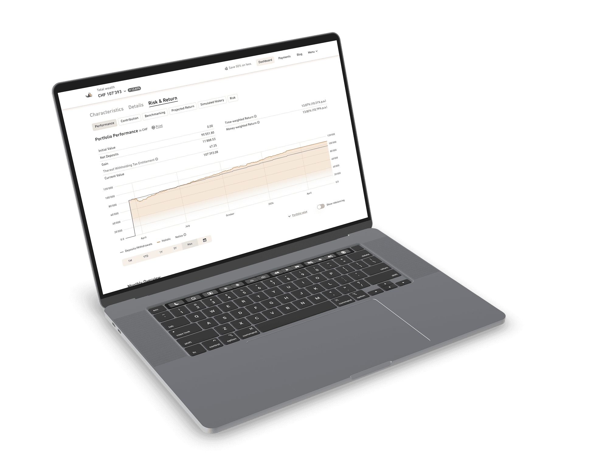
In addition to the deposits made, the gross profit, and the current portfolio value, the total Swiss Anticipatory Tax and foreign withholding tax have also been shown in an additional line since July 2025.
This shows the proportion of the profit generated that is attributable to anticipatory and withholding tax claims. If you use our free e-tax statement, you can apply for these tax refunds easily and without any red tape. Read more in our blog: «Greater transparency in terms of performance.»
About the author

Nicole is a Software Engineer at True Wealth.
Ready to invest?
Open accountNot sure how to start? Open a test account and upgrade to a full account later.
Open test account